XMATCH in Excel explained through examples
XMATCH is a useful function to get insight into even hefty Excel tables. With XMATCH, you can search and compare ranges of cells for a specific data element and find its relative position.
How does the XMATCH Excel function work?
You can use the XMATCH function to look through and compare data and items in a specific cell range. The only condition is that the cell range you’re looking through is a maximum of one column wide or one row high. The relative position that XMATCH shows you doesn't relate to the range of rows and columns in the whole table but rather to the relative position of the range of cells you have selected. The data you are looking for can be numerical or text. The function always ends after its search and will only ever give one position.
Just like the very recently added XLOOKUP feature, XMATCH is currently only available in Excel for Office 365 (status: September 2021).
XMATCH is basically an update to the existing MATCH function. XMATCH is an extension to MATCH with new search features that let you search not only from top to bottom (or left to right) but also in the other direction.
XMATCH syntax explained
Before you use the XMATCH feature, it’s worth making sure you know the arguments and syntax of the formula. The syntax for the XMATCH function always uses a lookup value and a lookup array. You can choose to add extra modes for the match and the search. The syntax of the XMATCH function works as follows:
=XMATCH(lookup_value, lookup_array, [match_mode], [search_mode])The arguments work as follows:
| Lookup value (required) | The data that the formula is looking for (e.g., text, number, wildcard) |
| Lookup array (required) | The cell range to search |
| Match mode (optional) | Defines the type of match for the search: 0 = Exact match -1 = Exact match or next smallest 1 = Exact match or next largest 2 = Wildcard match |
| Search mode (optional if match mode is given) | Defines the type of search: 1 = Search from first -1 = Search from last 2 = Binary search ascending (only if properly sorted) -2 = Binary search descending (only if properly sorted) |
Ways to use XMATCH
The XMATCH function in Excel offers a practical search function to find, compare and search through targeted data in organized lists. As an example, you can sort through, compare and analyze lists of employees or customers using specific search criteria. In large lists, you can even find out how many people have exceeded a certain criteria threshold for sales, or whether a specific quota has been met or undershot. Naturally, XMATCH lets you do lots of other things in Excel, too.
XMATCH in Excel explained through examples
Example 1: a simple comparison analysis of data
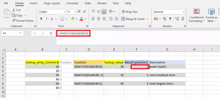
The example below should demonstrate the most basic feature of XMATCH. In the “lookup value” column, you can see what the function is looking for. In the “result” column, the result of the search through the cell range in “lookup array column B” is shown. The “description” shows you what the search result means.
Example 2: a concrete comparison analysis
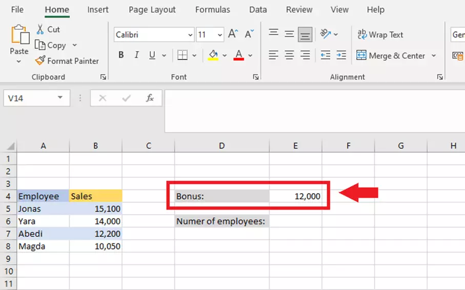
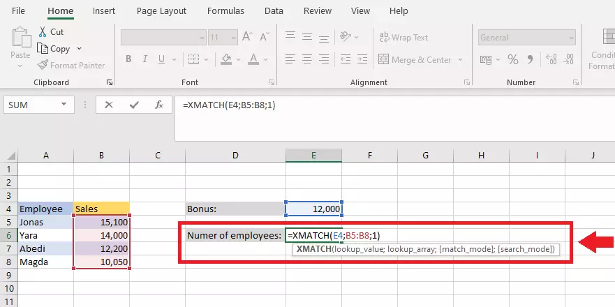
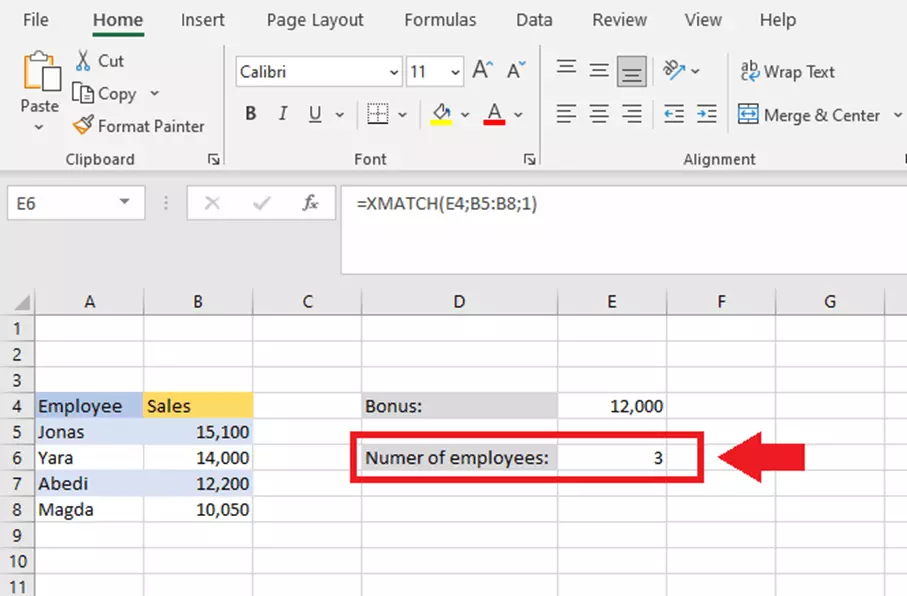
In the next example, XMATCH should show you how many employees in a given department will receive a bonus. To do this, match mode “1” must be used to find employees that exactly meet or exceed the search criteria and are therefore eligible for a bonus. For match mode “1” to work, the values must be listed in descending order.
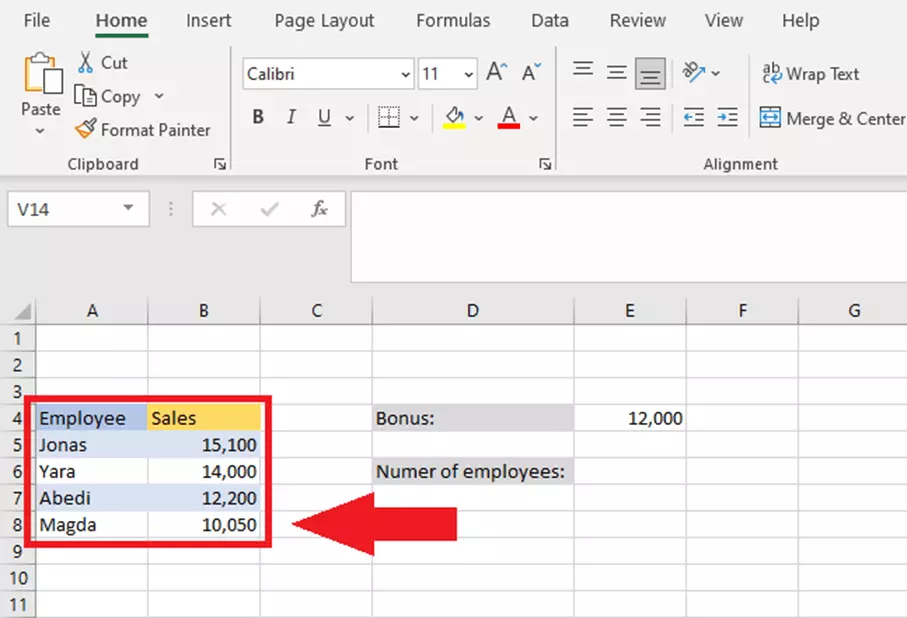
Step 1: Make a column with the names of the employees and a column with values in descending order.


