How to find and highlight duplicates in Excel
When working with complex tables, it’s rather difficult and time-consuming to find and highlight duplicate entries manually. Whether you are trying to identify an error in your data or simply want to analyze identical values in different cells, it’s helpful to know how to find duplicates in Excel.
How to identify duplicate values in Excel quick guide
- Go to Home and select the area in your Excel table that should be checked for duplicates.
- Click on Conditional Formatting.
- Click on Highlight Cell Rules and then on Duplicate Values….
- Now, choose how you want the duplicate cells to be formatted.
- Store, share, and edit data easily
- Backed up and highly secure
- Sync with all devices
How to find and format duplicates in Excel
Typically, you may want to find duplicates in Excel for one of the following reasons:
- They are there by mistake and should be deleted.
- All duplicates are important for analysis and should be highlighted in Excel.
The instructions presented below can be used with Excel version 2021, 2019 and 2016 as well as with the Microsoft 365 version of Excel.
Find out how to remove duplicates from datasets in our dedicated article on the topic.
Finding duplicates in Excel
With Excel, you don’t need to go through every single row yourself to find duplicates. The spreadsheet program can automatically display duplicates for you. To do so, you first need to select the area you want to check. This could be an entire row or column, or an area that you define yourself. You can use your mouse to select an area by dragging the square box. You can also select individual cells by simply holding down the Ctrl key and then clicking on the relevant cells.
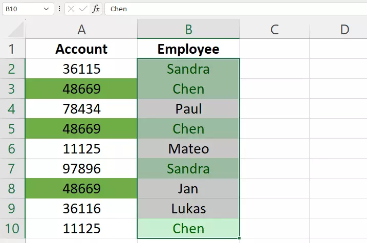
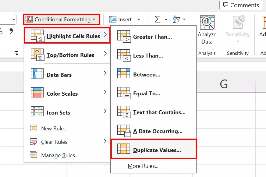
Once you have selected the area you want to analyze, you can use the conditional formatting feature in Excel to show duplicate values. To do this, follow the steps below:
- Go to Home.
- Click on Conditional Formatting in the Styles section.
- Select Highlight Cell Rules and then Duplicate Values.
After you’ve selected Duplicate Values…, you’ll be given the option to select the color that should be used to highlight the duplicates.
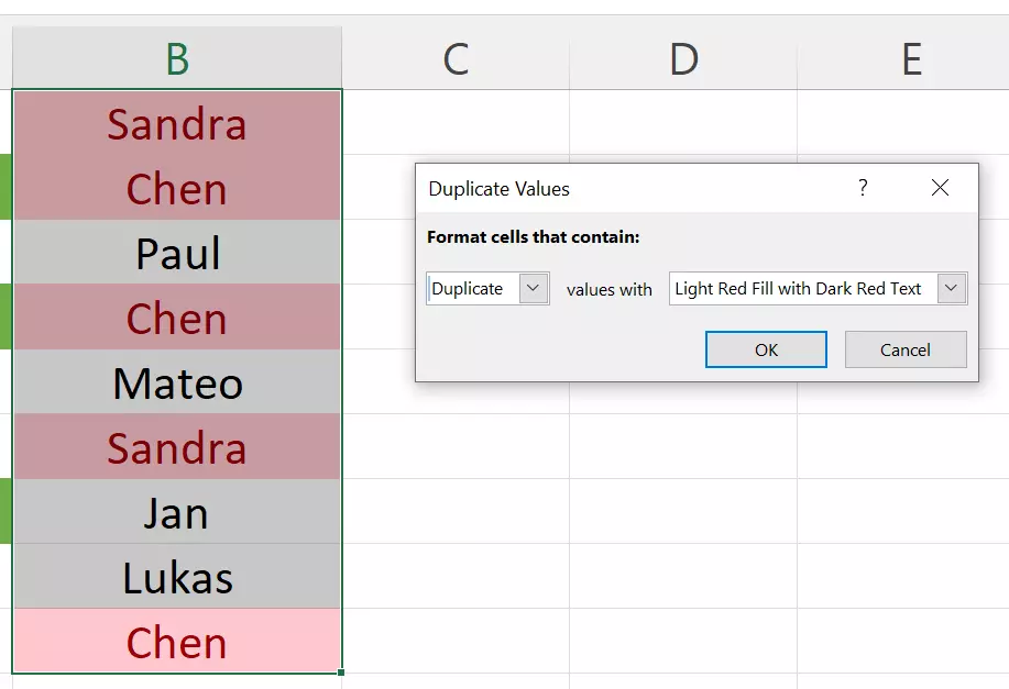
In addition to highlighting duplicates in Excel, you can also check for unique entries. To do so, select the option Unique from the drop-down menu on the left side of the Duplicate Values dialog box. Once you click OK, Excel will highlight all values that only appear once in the area you have selected.
Finding values that appear a specific number of times
With the Duplicate Values feature, all entries that appear more than once are highlighted. This includes values that appear three or four times. If you, for example, only want to find values that appear three times in a table, you can do this by creating a new rule and using the COUNTIF function:
- Open the Conditional Formatting menu und click on New Rule.
- Select the option Use a formula to determine which cells to format.
- Now, you need to enter a formula for the area in your table that you want to check. In our example, we’ll be using the following formula:
=COUNTIF($A$2:$A$10,A2)=3to check if there is a value that appears three times in the selected cells in column A. - Click on Format and select the formatting options you want to use to highlight values that appear three times.
- Click on OK to save the rule and apply it to your table.
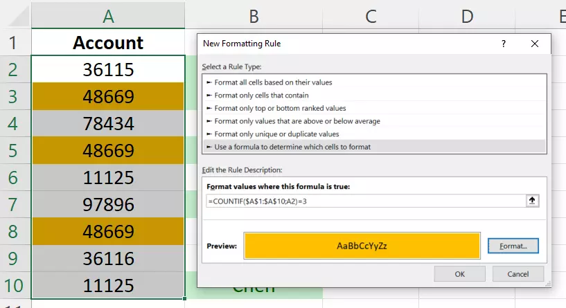
The COUNTIF function uses two parameters. The first parameter indicates the area that should be analyzed. The second parameter specifies the first cell of the area. The =3 at the end ensures that only those cells are formatted that contain a value that appears three times in the selected area.
With HiDrive cloud storage from IONOS, you can safely save, share and edit Office documents in one central location. Whether for private or professional use, you’ll be able to flexibly work from any device with the HiDrive app as well as with other interfaces. With state-of-the-art data centers, your data is securely protected.
Hiding other values when checking duplicates in Excel
You can also go a step further and hide all values that aren’t duplicates. Follow the steps below to use the filter function for the workbook you are using:
- Select the column that you want to use the filter feature for.
- In the ribbon, click on Data.
- Click on Filter in the Sort and Filter section.
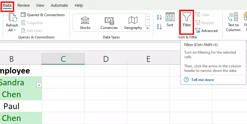
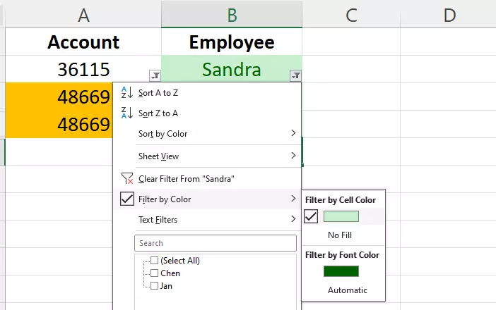
The first cell of the column will then show a drop-down menu where you can decide how to filter the data. Since we color-coded all duplicate values in the previous steps, all we have to do now is use the colors to filter the values. Once you have selected the filter criteria, Excel will only show duplicates, and all other values will be hidden.
You’ll encounter many other challenges when working with Excel on a daily basis. Find out about the most important Excel tricks and tips in our other articles:

