How to remove blank rows in Excel
When you start to create an Excel spreadsheet, you might not always have an exact structure in mind. After some reworking, you may end up with some blank rows in the spreadsheet and want to get rid of them as quickly and easily as possible. Fortunately, it’s not difficult to automatically remove blank rows in Excel.
The following instructions apply to Microsoft 365 and Excel versions 2021, 2019 and 2016.
Quick guide on how to remove blank rows in Excel
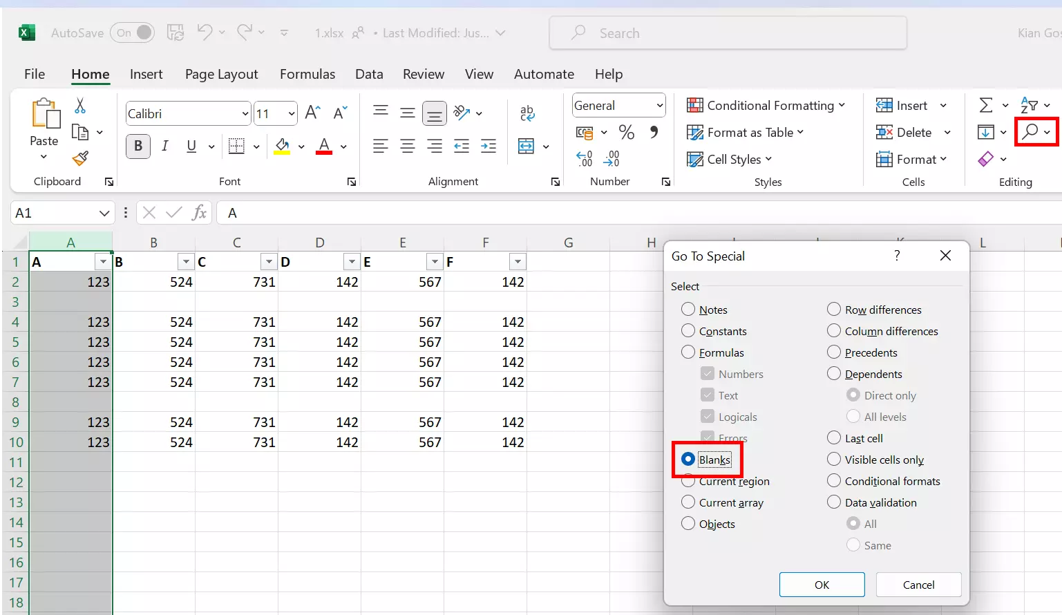
- Select a column in the table and then use the Go To… function under the Search and Select menu item.
- Click on Select and select Blanks to automatically select all empty cells.
- In the Home tab, click on Delete Cells…. If you select Entire row, Excel will remove the entire row where the program found a blank cell.
- Store, share, and edit data easily
- Backed up and highly secure
- Sync with all devices
Use the search feature in Excel to remove blank rows
The easiest way to delete all empty rows in Excel is with the built-in search function. To do this, select any column in your Excel spreadsheet and then use the Go To… feature under Find and Select.
A window should open. Click the Select button to access the selection menu. Here you can select Blanks. Now Excel should automatically select all empty cells in the selected column.

In the Home tab, you will find the option Delete Cells… under the option Delete. If you now click Entire row, Excel will remove the entire row where the program found an empty cell. It is important not to click outside of the marked area while you are doing this.

With IONOS HiDrive cloud storage, you can store, edit and share your Office documents centrally and securely. Whether for private or professional use, you can work flexibly from any device with the HiDrive app and other interfaces. Your data is optimally protected in state-of-the-art IONOS data centers.
Use filters to hide or remove blank rows
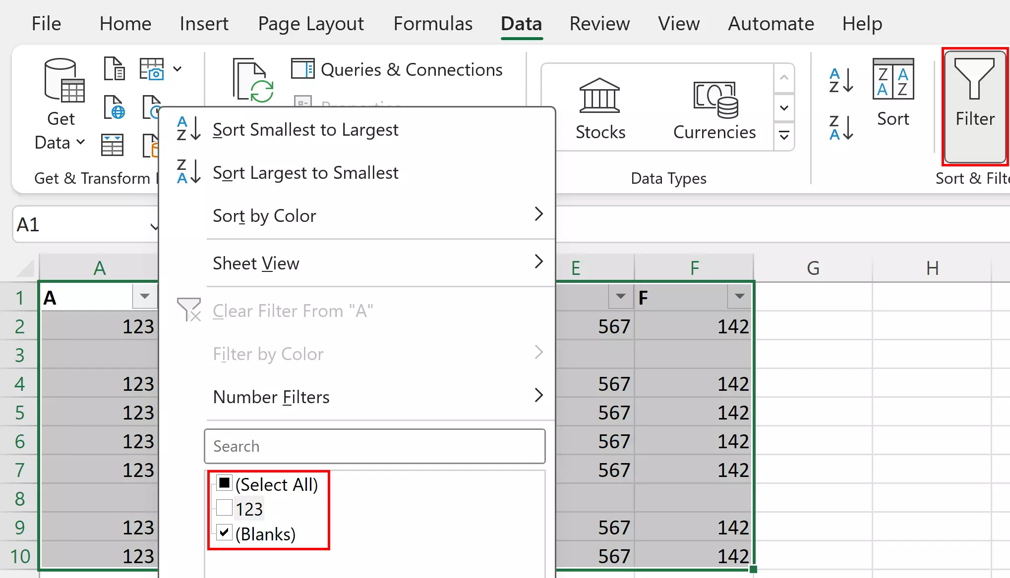
Not only can you use the search function to remove blank rows, you can also use a filter instead. To do this, mark the area where you want the blank rows removed. In the Data tab, you will find the Filter function. Clicking on the button creates a filter for each of the selected columns.
Excel generates a drop-down menu in the header row. There you can select which content should be displayed. One option is (Blanks). If you uncheck this option, Excel will hide all the blank rows.

To learn how to move columns and rows in Excel, see our article on this topic.
But you can also use the filter menu to show all empty rows. The blue text on the left side indicates which of the rows belong to the selected filtered area and where the actual table ends. Now highlight all the empty rows that are marked blue and then remove them.
Now open the filter’s Excel drop-down menu again. You should no longer be shown the (Blanks) option and should be able to show all the rows containing data again.


