Excel: Subtotals for your calculations

Microsoft’s spreadsheet program lets you produce comprehensive tables and complex calculations. Functions in Excel can assist in many situations and are rarely affected by the design and appearance of your tables. Want to hide certain cells for clarity? No problem: The functions still count the filtered values. However, you may not always want that. If you want your calculations to react to filters and hidden cells, the SUBTOTAL function is quite useful. It combines multiple calculation operations and gives you more control over the cells Excel includes.

You may not always want to see all cells, especially if you are working with large volumes of data. You can hide rows or certain values in order to make it easier to work with comprehensive tables. This reduces tables to a size that only shows the essential data, which makes it far simpler to work with them. However, the hidden values are not lost – they are still part of the worksheet and are therefore still used for calculation functions. That is a major advantage of Excel.

But what is generally an advantage can also be a problem in some situations. For example, if you want the Excel functions to react to what is currently visible and adapt your results accordingly, you can’t do so with the normal calculation methods. You would have to create a new table that does not include the values that are filtered out. The SUBTOTAL function gives you an alternative: You can configure the function to prevent hidden cells being included in the calculation.

SUBTOTAL combines no less than eleven different functions: Users choose which calculation method is to be used in the function, and whether to include hidden cells or not. The function does not include values currently hidden by a filter in the calculations. Accordingly, SUBTOTAL is ideal as an additional result to complement the final result. Comparing the two values often gives additional information.

Theoretically, the SUBTOTAL only needs two items of information. First, specify which calculation is to be performed. The second and all following arguments contain information on the range of cells used. One entry is required, but you can add up to 254 ranges to the formula.

The first parameter transfers the properties of another function to the SUBTOTAL function – Excel provides a list of functions. You enter the corresponding number and SUBTOTAL performs the corresponding calculation. However, there are two numbers for every function. Values between 1 and 11 configure SUBTOTAL to include hidden values. If you enter 101 to 111, the function ignores hidden cells in the specified range. Here is an overview.

Hidden cells remain part of the calculation:

• 1: AVERAGE
• 2: COUNT
• 3: COUNTA
• 4: MAX
• 5: MIN
• 6: PRODUCT
• 7: STDEV
• 8: STDEVP
• 9: SUM
• 10: VAR
• 11: VARP

Hidden cells are not included in calculations:

• 101: AVERAGE
• 102: COUNT
• 103: COUNTA
• 104: MAX
• 105: MIN
• 106: PRODUCT
• 107: STDEV
• 108: STDEVP
• 109: SUM
• 110: VAR
• 111: VARP

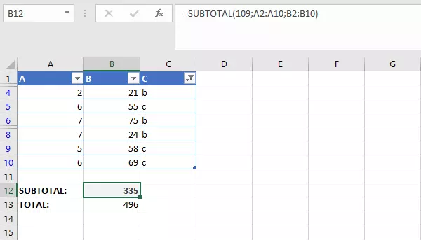
Calculating a sum is the best example of the SUBTOTAL function. Besides the final result including all values, the function also lets you calculate only the values not affected by filters or hidden values.

In this example, we take values from two columns and add them. As we entered 109 for the first parameters, only values that are currently visible are included.

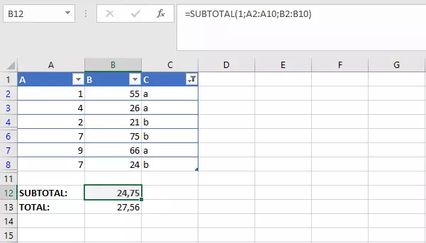
The same settings work with other calculation methods. For example, you can calculate the average.

You can also combine SUBTOTAL with other functions. Accordingly, the result of the function can be passed on directly to other calculations – without requiring auxiliary cells. For example, you can add up multiple subtotals.

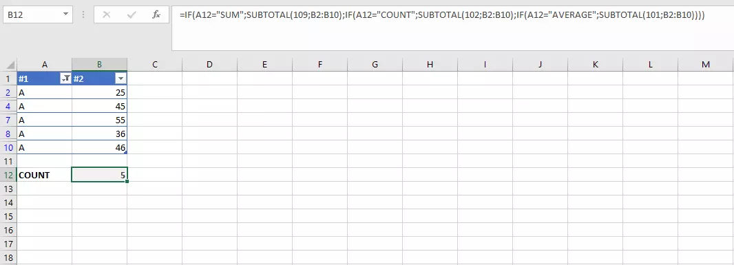
It can also be helpful to combine SUBTOTAL with the IF function. You can set up a cell in which you specify the required calculation type – for example using a drop-down menu. While that makes the formula itself somewhat longer, once you write it you never have to edit it afterwards. For example, if we assume that you want to switch between the three calculations SUM, COUNT and AVERAGE regularly.

Use AutoFilter to set the data that to be incorporated, and choose the required calculation from the dropdown list. The IF queries then always run the correct SUBTOTAL function.

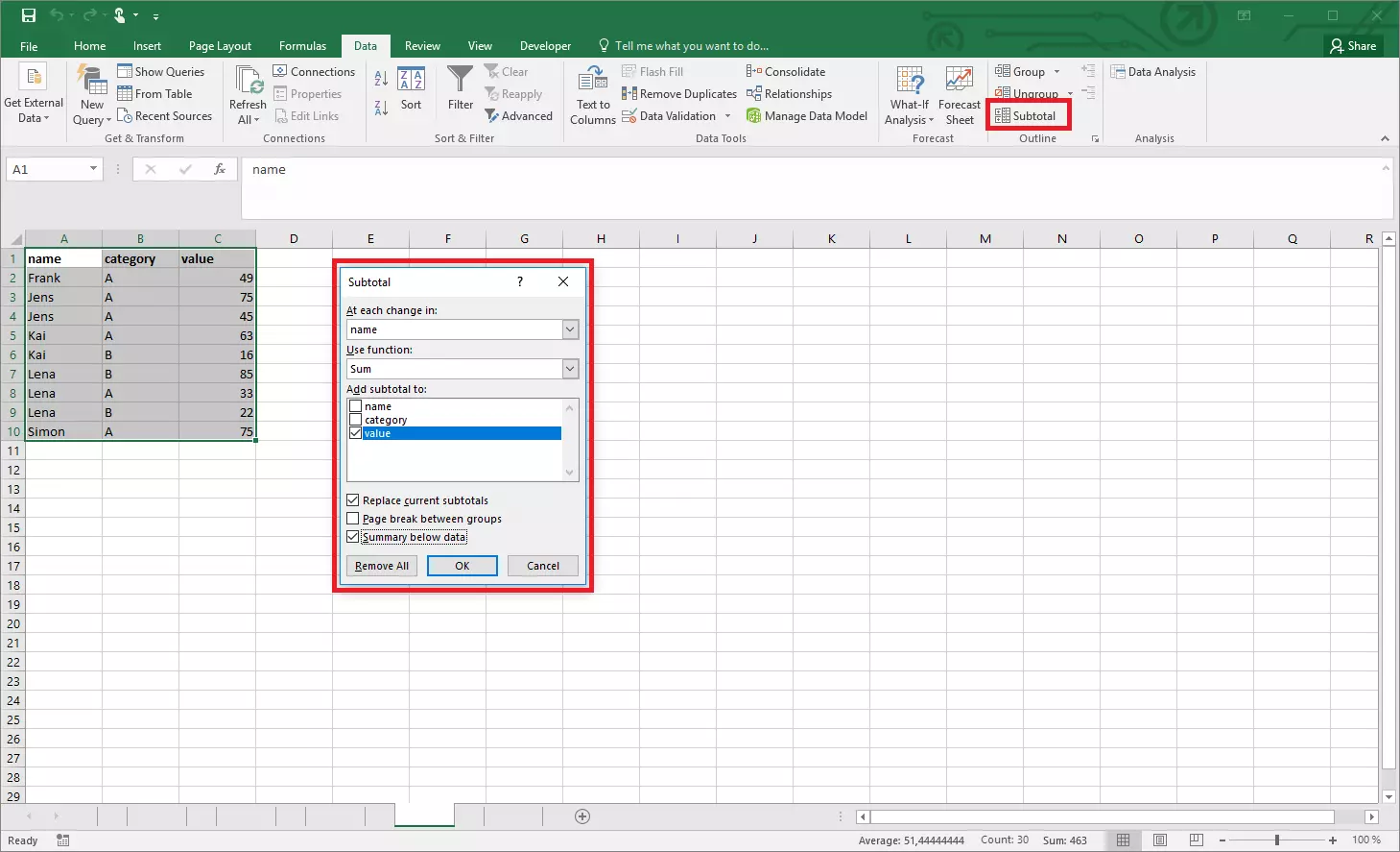
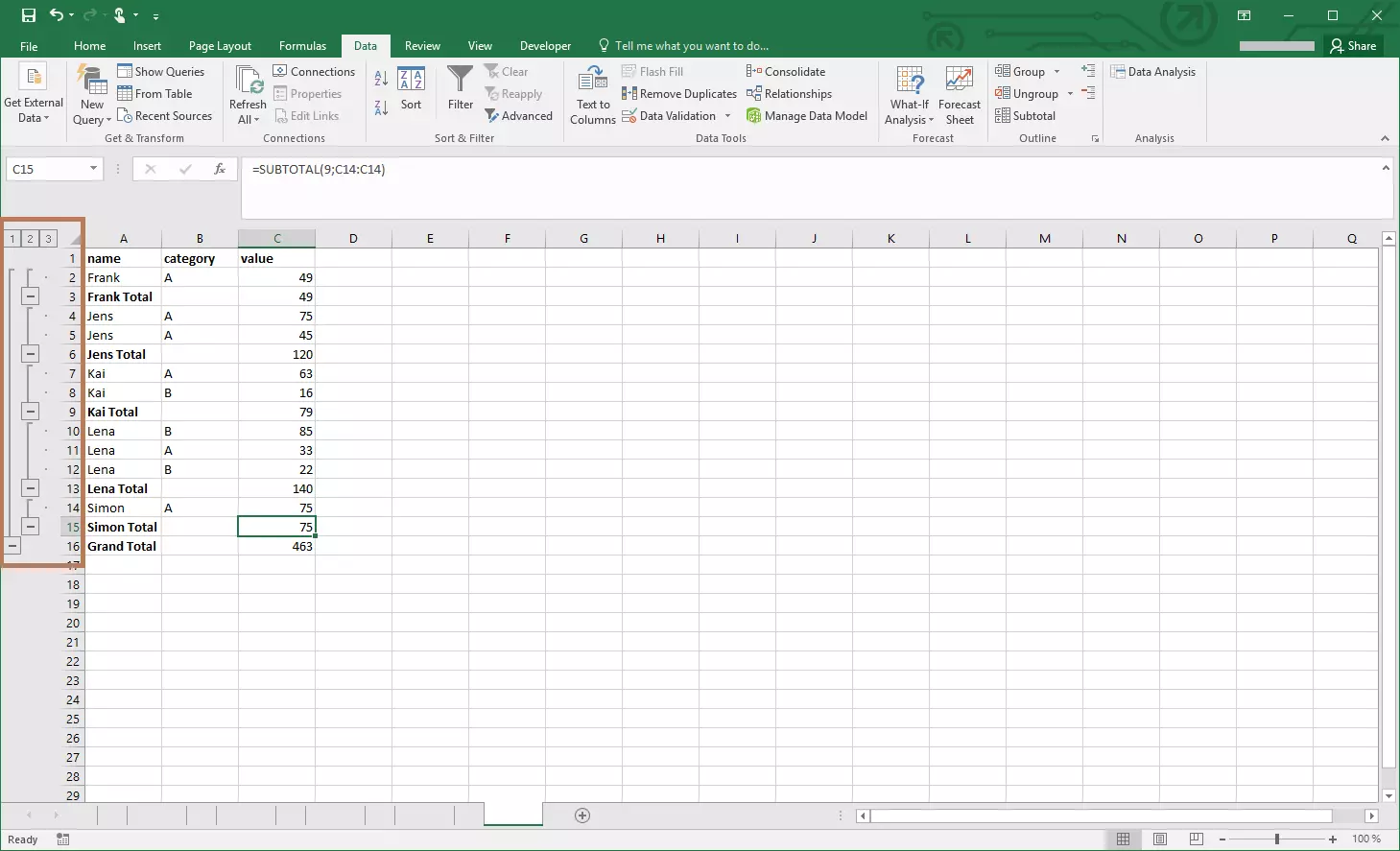
Besides the function, which is easy to integrate in formulas, Excel offers another tool of the same name. You can find it in the “Data” tab under the “Subtotal” button. This tool is useful if you have a multi-column list in Excel, for example. You can include a fixed set of values (generally non-numerical) – for example names – in one column. In turn, these entries are assigned to numerical values: revenues, point scores, measurements and similar data. The tool helps you calculate subtotals from groups – all identical entries in one column are grouped and the corresponding values in the other column are calculated.