How to create and edit pivot tables in Google Sheets

In Google Sheets, you can create a pivot table to manage large datasets effectively. You control how data is restructured and filtered so you can display the data precisely and according to what you need. To be able to use pivot tables in Google Sheets, you need to make sure all the columns in your table have a heading.

What are the requirements for creating a Google Sheets pivot table?

To create a pivot table in Google Sheets, each column in the document needs to have its own heading. These headings serve as filtering options and can be included or excluded in the pivot tables. You can then determine which order data should be displayed in and how it should be filtered.

How to create a pivot table in Google

You can create a pivot table in Google Sheets with just a few clicks. Simply follow these steps:

1. Open the document that you want to create a pivot table from.
2. Click anywhere inside the table.
3. Select the Insert option at the top of the tab and then Pivot table.

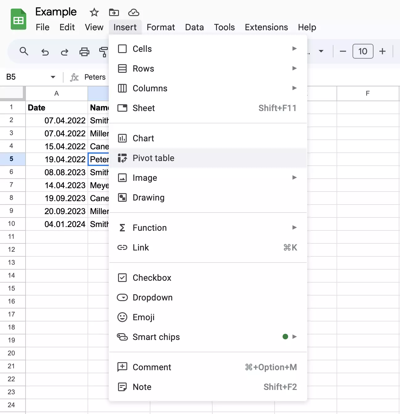
4. A window will now open. Under Data range, specify which part of the table you want the pivot table to take into account.
5. You’ll be asked where you would like to insert the pivot table. It’s best to create this in a new worksheet. You can also continue working in the existing worksheet if you prefer.
6. Click Create. Now, you’ll automatically be switched to your new pivot table.

Working with Google Sheets pivot tables

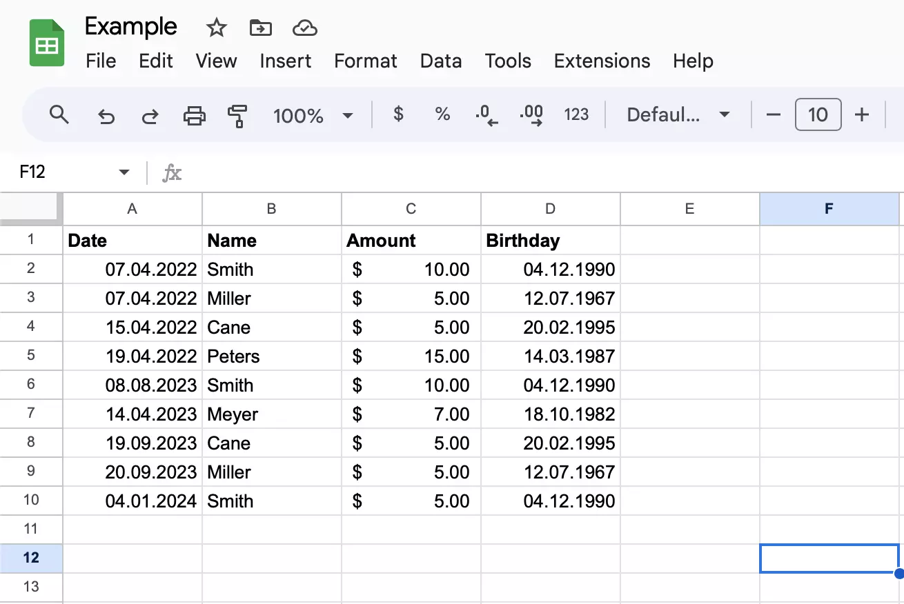
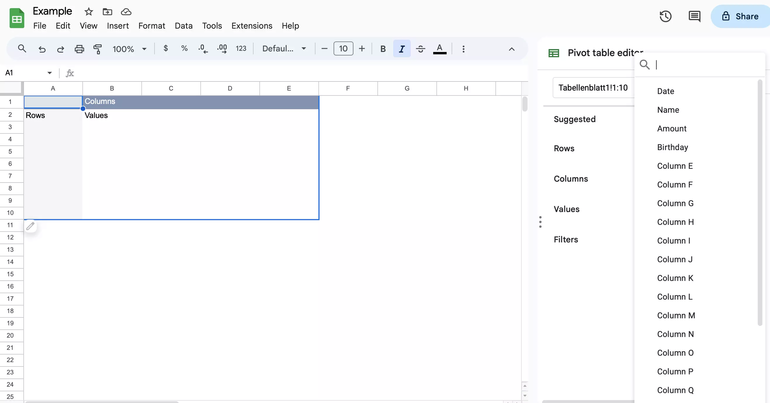
You’ll receive an empty pivot table in Google Sheets, which you can edit using the editor. Four parameters are at your disposal: Rows, Columns, Values and Filters. We’ll explain how to use these below. In our example, several people have contributed various amounts of money into a money pool on different days. We have created a table for the money pool, which includes everyone’s birthdays, in addition to their names, the amount they contributed and when they contributed the money. We’ll now use the pivot table to filter this information according to what we need.

How to sort a pivot table by row

First, we want to sort the entire content row by row according to each individual person and then determine how much money has been deposited in total. We can do this in just a few steps:

1. Click on Add next to the Rows option.
2. Then click on Name.

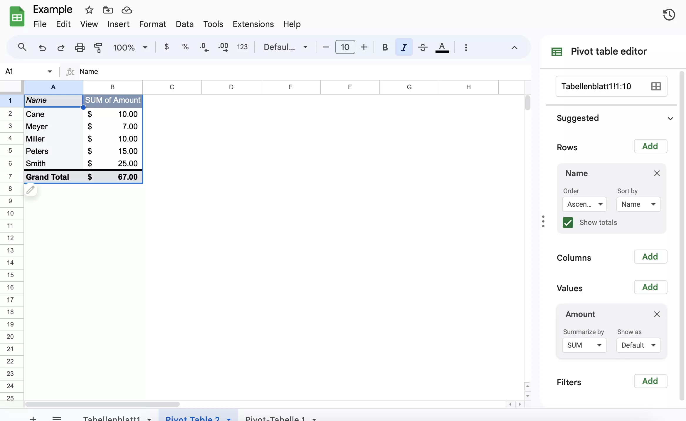
3. Specify the order and decide whether the total number should be displayed.
4. Select Values by clicking on Add again.
5. In the Amount section, you can now see how much each person has paid as well as the total amount in the money pool. You can also find out other values by clicking on the arrow under Summarize by.

How to sort a pivot table by date

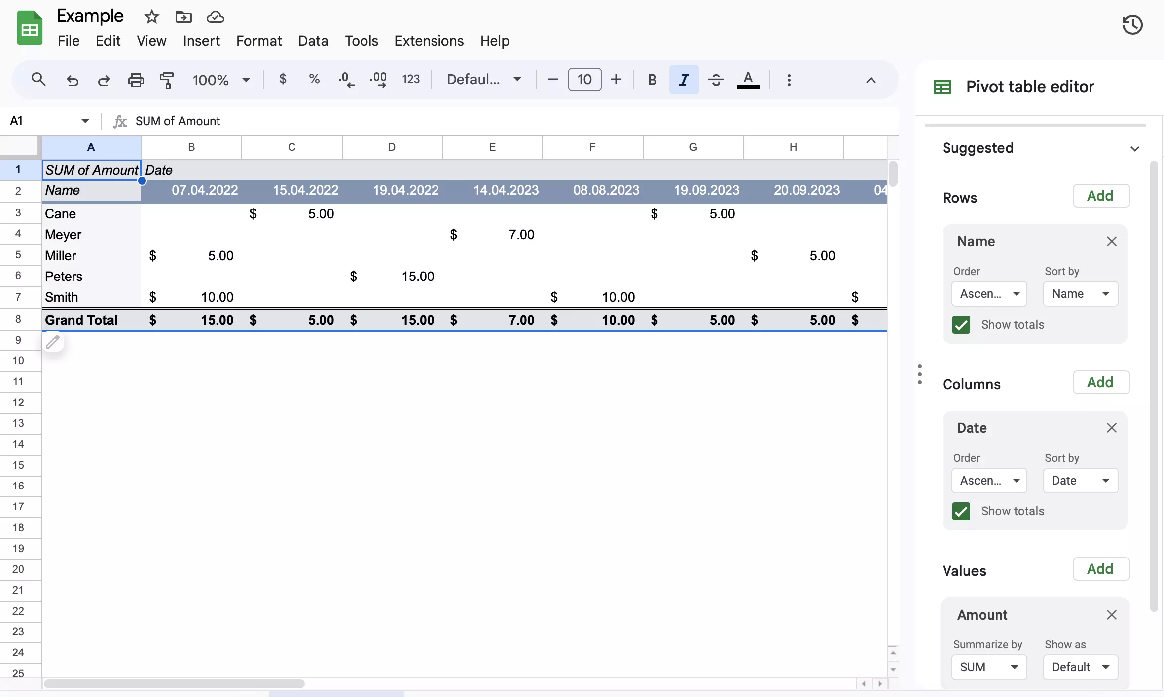
Next, we want to show which amounts were paid into the money pool on which days. The dates of birth are unimportant and can be filtered out. This is just one example of how useful Google Sheet’s pivot tables can be. We also want to see who paid money when. In the example below, we’re going to sort the values column by column:

1. First, click on Add in the Columns section and select Date. All the dates where at least one person made a deposit will be displayed next to each other.
2. Next, click on Add in the Rows section and select Name. This gives you the finished structure of your pivot table. Now, all the table needs is values.
3. Click on Add in the Values section and select Amount. You’ll now see the total amount deposited per day at the bottom, a summary of the amounts paid by each individual on the right, and the total amount currently in the money pool in the bottom right-hand corner of the table.

The more extensive your table is, the more it makes sense to create a pivot table in Google Sheets. You can add or hide additional parameters using the Filter option.